How To Parametrize A Plane

x.1: Parametrizations of Plane Curves

Last updated
Save as PDF

Folio ID: 8192

Learning Objectives

Plot a curve described by parametric equations.
Convert the parametric equations of a curve into the form $y=f(x)$.
Recognize the parametric equations of bones curves, such as a line and a circle.
Recognize the parametric equations of a cycloid.

In this section we examine parametric equations and their graphs. In the two-dimensional coordinate system, parametric equations are useful for describing curves that are non necessarily functions. The parameter is an independent variable that both $ten$ and $y$ depend on, and as the parameter increases, the values of $x$ and $y$ trace out a path forth a plane curve. For example, if the parameter is $t$ (a common choice), then $t$ might represent time. So $x$ and $y$ are divers as functions of time, and $(x(t),y(t))$ can depict the position in the plane of a given object every bit it moves along a curved path.

Parametric Equations and Their Graphs

Consider the orbit of World around the Sun. Our yr lasts approximately 365.25 days, only for this discussion we will utilise 365 days. On January 1 of each yr, the physical location of Earth with respect to the Dominicus is nearly the same, except for spring years, when the lag introduced by the extra $\frac{i}{4}$ 24-hour interval of orbiting time is congenital into the calendar. We call January i "twenty-four hours 1" of the year. Then, for example, solar day 31 is January 31, mean solar day 59 is February 28, so on.

The number of the day in a twelvemonth can be considered a variable that determines Earth'southward position in its orbit. Every bit Globe revolves effectually the Sun, its physical location changes relative to the Dominicus. After one full year, we are back where we started, and a new year begins. Co-ordinate to Kepler's laws of planetary motility, the shape of the orbit is elliptical, with the Sun at one focus of the ellipse. We study this thought in more detail in Conic Sections.

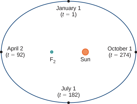
An ellipse with January 1 (t = 1) at the top, April 2 (t = 92) on the left, July 1 (t = 182) on the bottom, and October 1 (t = 274) on the right. The focal points of the ellipse have F2 on the left and the Sun on the right. — Figure $\PageIndex{one}$: Earth's orbit around the Sun in one year.

Figure $ \PageIndex{1}$ depicts Earth's orbit around the Dominicus during 1 year. The indicate labeled $F_2$ is one of the foci of the ellipse; the other focus is occupied by the Sun. If we superimpose coordinate axes over this graph, then nosotros can assign ordered pairs to each point on the ellipse (Effigy $ \PageIndex{2}$). Then each $x$ value on the graph is a value of position as a function of time, and each $y$ value is besides a value of position as a function of fourth dimension. Therefore, each point on the graph corresponds to a value of Earth'due south position as a function of time.

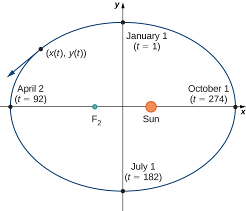
We can make up one's mind the functions for $10(t)$ and $y(t)$, thereby parameterizing the orbit of Earth around the Lord's day. The variable $t$ is called an independent parameter and, in this context, represents time relative to the beginning of each year.

A bend in the $(ten,y)$ plane can be represented parametrically. The equations that are used to define the bend are called parametric equations.

Definition: Parametric Equations

If $x$ and $y$ are continuous functions of $t$ on an interval $I$, then the equations

\[ten=10(t) \nonumber \]

and

\[y=y(t) \nonumber \]

are called parametric equations and $t$ is chosen the parameter. The set of points $(10,y)$ obtained as $t$ varies over the interval $I$ is called the graph of the parametric equations. The graph of parametric equations is called a parametric bend or airplane bend, and is denoted by $C$.

Notice in this definition that $x$ and $y$ are used in 2 ways. The first is equally functions of the contained variable $t$. As $t$ varies over the interval $I$, the functions $ten(t)$ and $y(t)$ generate a prepare of ordered pairs $(x,y)$. This set up of ordered pairs generates the graph of the parametric equations. In this second usage, to designate the ordered pairs, $x$ and $y$ are variables. It is important to distinguish the variables $x$ and $y$ from the functions $x(t)$ and $y(t)$.

Case $\PageIndex{one}$: Graphing a Parametrically Divers Curve

Sketch the curves described by the following parametric equations:

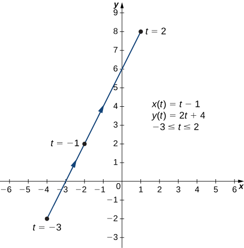
$ten(t)=t−ane, \quad y(t)=2t+4,\quad \text{for }−3≤t≤ii$
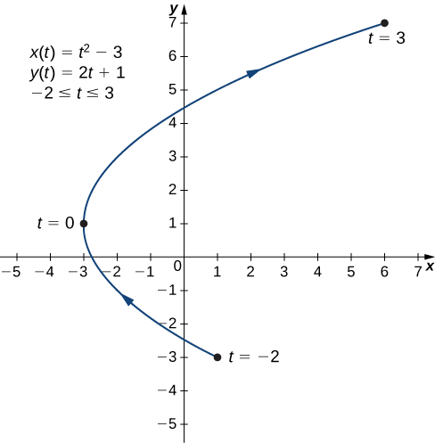
$x(t)=t^2−iii, \quad y(t)=2t+1,\quad \text{for }−2≤t≤iii$
$x(t)=iv \cos t, \quad y(t)=4 \sin t,\quad \text{for }0≤t≤2π$

Solution

a. To create a graph of this curve, starting time ready a table of values. Since the independent variable in both $ten(t)$ and $y(t)$ is $t$, permit $t$ appear in the start column. Then $x(t)$ and $y(t)$ will appear in the second and third columns of the table.

$t$	$x(t)$	$y(t)$
−3	−4	−2
−2	−3	0
−one	−2	2
0	−1	4
1	0	six
two	1	eight

The second and tertiary columns in this tabular array provide a set of points to be plotted. The graph of these points appears in Effigy $ \PageIndex{3}$. The arrows on the graph bespeak the orientation of the graph, that is, the direction that a indicate moves on the graph as t varies from −3 to two.

A straight line going from (−4, −2) through (−3, 0), (−2, 2), and (0, 6) to (1, 8) with arrow pointed up and to the right. The point (−4, −2) is marked t = −3, the point (−2, 2) is marked t = −1, and the point (1, 8) is marked t = 2. On the graph there are also written three equations: x(t) = t −1, y(t) = 2t + 4, and −3 ≤ t ≤ 2. — Figure $\PageIndex{3}$: Graph of the plane curve described by the parametric equations in part a.

b. To create a graph of this bend, again gear up a table of values.

$t$	$x(t)$	$y(t)$
−2	1	−3
−1	−2	−1
0	−three	1
1	−2	3
2	1	5
iii	6	7

The second and third columns in this table requite a set of points to be plotted (Figure $ \PageIndex{four}$). The first point on the graph (respective to $t=−2$) has coordinates $(1,−3)$, and the terminal point (corresponding to $t=three$) has coordinates $(6,7)$. As $t$ progresses from $−2$ to $3$, the point on the curve travels forth a parabola. The direction the point moves is once more called the orientation and is indicated on the graph.

A curved line going from (1, −3) through (−3, 1) to (6, 7) with arrow pointing in that order. The point (1, −3) is marked t = −2, the point (−3, 1) is marked t = 0, and the point (6, 7) is marked t = 3. On the graph there are also written three equations: x(t) = t2 − 3, y(t) = 2t + 1, and −2 ≤ t ≤ 3. — Figure $\PageIndex{4}$: Graph of the plane curve described by the parametric equations in function b.

c. In this case, apply multiples of $π/half dozen$ for $t$ and create some other table of values:

$t$	$x(t)$	$y(t)$	$t$	$ten(t)$	$y(t)$
0	4	0	$\frac{7π}{6}$	$-ii\sqrt{3}≈−iii.v$	-2
$\frac{π}{6}$	$2\sqrt{three}≈3.5$	two	$\frac{4π}{3}$	−ii	$−2\sqrt{iii}≈−3.five$
$\frac{π}{3}$	2	$2\sqrt{three}≈3.5$	$\frac{3π}{2}$	0	−4
$\frac{π}{ii}$	0	4	$\frac{5π}{3}$	2	$−2\sqrt{3}≈−three.5$
$\frac{2π}{three}$	−ii	$2\sqrt{3}≈3.5$	$\frac{11π}{6}$	$two\sqrt{3}≈3.5$	-2
$\frac{5π}{six}$	$−two\sqrt{iii}≈−three.5$	2	$2π$	4	0
$π$	−4	0

The graph of this plane bend appears in the following graph.

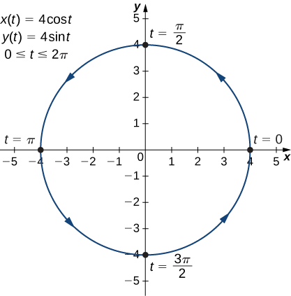
A circle with radius 4 centered at the origin is graphed with arrow going counterclockwise. The point (4, 0) is marked t = 0, the point (0, 4) is marked t = π/2, the point (−4, 0) is marked t = π, and the point (0, −4) is marked t = 3π/2. On the graph there are also written three equations: x(t) = 4 cos(t), y(t) = 4 sin(t), and 0 ≤ t ≤ 2π. — Effigy $\PageIndex{5}$: Graph of the airplane curve described past the parametric equations in function c.

This is the graph of a circle with radius $4$ centered at the origin, with a counterclockwise orientation. The starting point and ending points of the curve both have coordinates $(4,0)$.

Exercise $\PageIndex{1}$

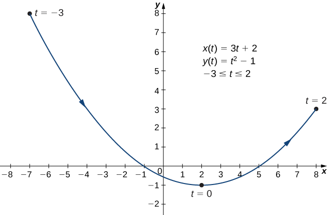
Sketch the bend described by the parametric equations

\[ x(t)=3t+2,\quad y(t)=t^two−one,\quad \text{for }−3≤t≤2. \nonumber \]

Hint: Make a table of values for $x(t)$ and $y(t)$ using $t$ values from $−three$ to $ii$.

Reply: $A curved line going from (−7, 8) through (−1, 0) and (2, −1) to (8, 3) with arrow going in that order. The point (−7, 8) is marked t = −3, the point (2, −1) is marked t = 0, and the point (8, 3) is marked t = 2. On the graph there are also written three equations: x(t) = 3t + 2, y(t) = t2 − 1, and −3 ≤ t ≤ 2.$

Eliminating the Parameter

To ameliorate understand the graph of a curve represented parametrically, it is useful to rewrite the two equations equally a single equation relating the variables $x$ and $y$. So we can apply any previous noesis of equations of curves in the plane to identify the curve. For example, the equations describing the aeroplane bend in Case $\PageIndex{1b}$ are

\[\begin{marshal} x(t) &=t^2−3 \label{x1} \\[4pt] y(t) &=2t+1 \characterization{y1} \terminate{align} \]

over the region $-2 \le t \le 3.$

Solving Equation \ref{y1} for $t$ gives

\[t=\dfrac{y−one}{2}. \nonumber \]

This tin can be substituted into Equation \ref{x1}:

\[\begin{align} x &=\left(\dfrac{y−i}{2}\right)^2−3 \\[4pt] &=\dfrac{y^2−2y+1}{four}−3 \\[4pt] &=\dfrac{y^2−2y−11}{4}. \label{y2}\terminate{align} \]

Equation \ref{y2} describes $x$ as a function of $y$. These steps requite an instance of eliminating the parameter. The graph of this role is a parabola opening to the right (Figure $\PageIndex{4}$). Recollect that the airplane bend started at $(1,−3)$ and concluded at $(six,7)$. These terminations were due to the brake on the parameter $t$.

Example $\PageIndex{2}$: Eliminating the Parameter

Eliminate the parameter for each of the plane curves described by the post-obit parametric equations and describe the resulting graph.

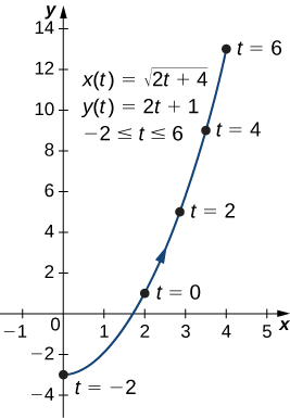
$10(t)=\sqrt{2t+iv}, \quad y(t)=2t+1,\quad \text{for }−2≤t≤half-dozen$
$x(t)=4\cos t, \quad y(t)=3\sin t,\quad \text{for }0≤t≤2π$

Solution

a. To eliminate the parameter, nosotros tin solve either of the equations for $t$. For example, solving the showtime equation for $t$ gives

\[\begin{align*} ten &=\sqrt{2t+4} \\[4pt] x^2 &=2t+4 \\[4pt] x^2−4 &=2t \\[4pt] t &=\dfrac{ten^two−4}{ii}. \end{align*}\]

Note that when we square both sides information technology is important to find that $ten≥0$. Substituting $t=\dfrac{x^2−4}{2}$ into $y(t)$ yields

\[ y(t)=2t+ane \nonumber \]

\[ y=2\left(\dfrac{x^2−iv}{2}\right)+one \nonumber \]

\[ y=x^two−4+1 \nonumber \]

\[ y=x^2−3. \nonumber \]

This is the equation of a parabola opening upward. There is, however, a domain restriction because of the limits on the parameter $t$. When $t=−two$, $x=\sqrt{ii(−two)+4}=0$, and when $t=6$, $ten=\sqrt{2(6)+4}=4$. The graph of this plane bend follows.

A curved line going from (−3, 0) through (2, 1) to (4, 13) with arrow going in that order. The point (−3, 0) is marked t = −2, the point (2, 1) is marked t = 0, the point (2 times the square root of 2, 5) is marked t = 2, the point (3 times the square root of 2, 9) is marked t = 4, and the point (4, 13) is marked t = 6. On the graph there are also written three equations: x(t) = square root of the quantity (2t + 4), y(t) = 2t + 1, and −2 ≤ t ≤ 6. — Figure $\PageIndex{6}$: Graph of the plane curve described by the parametric equations in part a.

b. Sometimes it is necessary to be a bit creative in eliminating the parameter. The parametric equations for this example are

\[ x(t)=4 \cos t\nonumber \]

and

\[ y(t)=3 \sin t\nonumber \]

Solving either equation for $t$ direct is not advisable because sine and cosine are not 1-to-1 functions. Nevertheless, dividing the commencement equation by $four$ and the 2d equation by $3$ (and suppressing the $t$) gives united states of america

\[ \cos t=\dfrac{x}{4}\nonumber \]

and

\[ \sin t=\dfrac{y}{three}.\nonumber \]

At present utilise the Pythagorean identity $\cos^2t+\sin^2t=1$ and supplant the expressions for $\sin t$ and $\cos t$ with the equivalent expressions in terms of $10$ and $y$. This gives

\[ \left(\dfrac{x}{4}\correct)^2+\left(\dfrac{y}{3}\correct)^two=1 \nonumber \]

\[ \dfrac{10^2}{16}+\dfrac{y^2}{ix}=1. \nonumber \]

This is the equation of a horizontal ellipse centered at the origin, with semi-major axis $four$ and semi-pocket-size axis $3$ equally shown in the following graph.

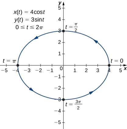
An ellipse with major axis horizontal and of length 8 and with minor radius vertical and of length 6 that is centered at the origin with arrow going counterclockwise. The point (4, 0) is marked t = 0, the point (0, 3) is marked t = π/2, the point (−4, 0) is marked t = π, and the point (0, −3) is marked t = 3π/2. On the graph there are also written three equations: x(t) = 4 cos(t), y(t) = 3 sin(t), and 0 ≤ t ≤ 2π. — Effigy $\PageIndex{7}$: Graph of the plane curve described by the parametric equations in part b.

As t progresses from $0$ to $2π$, a point on the curve traverses the ellipse once, in a counterclockwise management. Call back from the section opener that the orbit of World around the Dominicus is also elliptical. This is a perfect example of using parameterized curves to model a existent-world phenomenon.

Exercise $\PageIndex{2}$

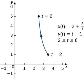
Eliminate the parameter for the plane curve defined by the following parametric equations and describe the resulting graph.

\[ x(t)=two+\dfrac{3}{t}, \quad y(t)=t−1, \quad\text{for }2≤t≤6 \nonumber \]

Hint: Solve one of the equations for $t$ and substitute into the other equation.

Respond

$10=ii+\frac{iii}{y+1},$ or $y=−1+\frac{3}{x−ii}$. This equation describes a portion of a rectangular hyperbola centered at $(ii,−ane)$.

$A curved line going from (3.5, 1) to (2.5, 5) with arrow going in that order. The point (3.5, 1) is marked t = 2 and the point (2.5, 5) is marked t = 6. On the graph there are also written three equations: x(t) = 2 + 3/t, y(t) = t − 1, and 2 ≤ t ≤ 6.$

And so far we accept seen the method of eliminating the parameter, bold we know a prepare of parametric equations that depict a plane curve. What if we would like to start with the equation of a curve and determine a pair of parametric equations for that curve? This is certainly possible, and in fact it is possible to do so in many different means for a given curve. The procedure is known as parameterization of a curve.

Case $\PageIndex{3}$: Parameterizing a Bend

Find ii different pairs of parametric equations to represent the graph of $y=2x^two−3$.

Solution

Start, it is always possible to parameterize a curve past defining $x(t)=t$, so replacing $x$ with $t$ in the equation for $y(t)$. This gives the parameterization

\[ 10(t)=t, \quad y(t)=2t^ii−3. \nonumber \]

Since there is no restriction on the domain in the original graph, there is no restriction on the values of $t$.

Nosotros have complete freedom in the selection for the second parameterization. For example, we can choose $x(t)=3t−ii$. The only thing we need to check is that there are no restrictions imposed on $x$; that is, the range of $x(t)$ is all real numbers. This is the instance for $10(t)=3t−2$. At present since $y=2x^2−three$, we can substitute $x(t)=3t−2$ for $x$. This gives

\[ y(t)=2(3t−two)^2−2=2(9t^2−12t+4)−2=18t^ii−24t+8−2=18t^ii−24t+6. \nonumber \]

Therefore, a second parameterization of the curve can be written equally

$ x(t)=3t−2$ and $ y(t)=18t^ii−24t+vi.$

Practice $\PageIndex{3}$

Find two different sets of parametric equations to represent the graph of $y=ten^ii+2x$.

Hint: Follow the steps in Example $\PageIndex{3}$. Remember we accept freedom in choosing the parameterization for $10(t)$.

Reply: One possibility is $x(t)=t, \quad y(t)=t^2+2t.$ Another possibility is $x(t)=2t−3, \quad y(t)=(2t−3)^2+two(2t−3)=4t^two−8t+3.$ There are, in fact, an infinite number of possibilities.

Cycloids and Other Parametric Curves

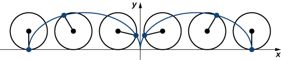
Imagine going on a bicycle ride through the country. The tires stay in contact with the road and rotate in a anticipated blueprint. Now suppose a very determined emmet is tired after a long day and wants to get home. So he hangs onto the side of the tire and gets a free ride. The path that this ant travels down a straight road is called a cycloid (Figure $ \PageIndex{eight}$). A cycloid generated by a circumvolve (or bicycle wheel) of radius a is given by the parametric equations

\[10(t)=a(t−\sin t), \quad y(t)=a(1−\cos t).\nonumber \]

To run into why this is true, consider the path that the center of the cycle takes. The eye moves along the $ten$-centrality at a abiding pinnacle equal to the radius of the bicycle. If the radius is $a$, then the coordinates of the middle can be given by the equations

\[x(t)=at,\quad y(t)=a\nonumber \]

for any value of $t$. Next, consider the ant, which rotates around the center along a circular path. If the bicycle is moving from left to correct then the wheels are rotating in a clockwise direction. A possible parameterization of the circular motion of the ant (relative to the center of the wheel) is given by

\[\begin{align*} x(t) &=−a \sin t \\[4pt] y(t) &=−a\cos t.\end{marshal*}\]

(The negative sign is needed to reverse the orientation of the curve. If the negative sign were not there, nosotros would have to imagine the wheel rotating counterclockwise.) Adding these equations together gives the equations for the cycloid.

\[\brainstorm{align*} 10(t) &=a(t−\sin t) \\[4pt] y(t) &=a(1−\cos t ) \end{align*}\]

A series of circles with center marked and a point on the circle drawing out a curve as if the circle was rolling along a plane. The shape made seems to be half an ellipse with height the diameter of the original circle and with major axis the circumference of the circle. — Figure $\PageIndex{8}$: A cycle traveling along a road without slipping; the point on the edge of the wheel traces out a cycloid.

At present suppose that the bicycle bike doesn't travel along a straight road but instead moves along the within of a larger bike, as in Figure $ \PageIndex{9}$. In this graph, the green circle is traveling around the blue circle in a counterclockwise direction. A indicate on the edge of the green circumvolve traces out the red graph, which is called a hypocycloid .

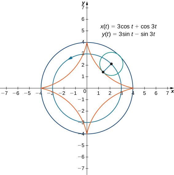
Two circles are drawn both with center at the origin and with radii 3 and 4, respectively; the circle with radius 3 has an arrow pointing in the counterclockwise direction. There is a third circle drawn with center on the circle with radius 3 and touching the circle with radius 4 at one point. That is, this third circle has radius 1. A point is drawn on this third circle, and if it were to roll along the other two circles, it would draw out a four pointed star with points at (4, 0), (0, 4), (−4, 0), and (0, −4). On the graph there are also written two equations: x(t) = 3 cos(t) + cos(3t) and y(t) = 3 sin(t) – sin(3t). — Effigy $\PageIndex{nine}$: Graph of the hypocycloid described by the parametric equations shown.

The general parametric equations for a hypocycloid are

\[ten(t)=(a−b) \cos t+b \cos (\dfrac{a−b}{b})t \nonumber \]

\[y(t)=(a−b) \sin t−b \sin (\dfrac{a−b}{b})t. \nonumber \]

These equations are a flake more than complicated, merely the derivation is somewhat similar to the equations for the cycloid. In this case we assume the radius of the larger circle is $a$ and the radius of the smaller circle is $b$. And then the center of the wheel travels along a circumvolve of radius $a−b.$ This fact explains the first term in each equation above. The period of the second trigonometric function in both $10(t)$ and $y(t)$ is equal to $\dfrac{2πb}{a−b}$.

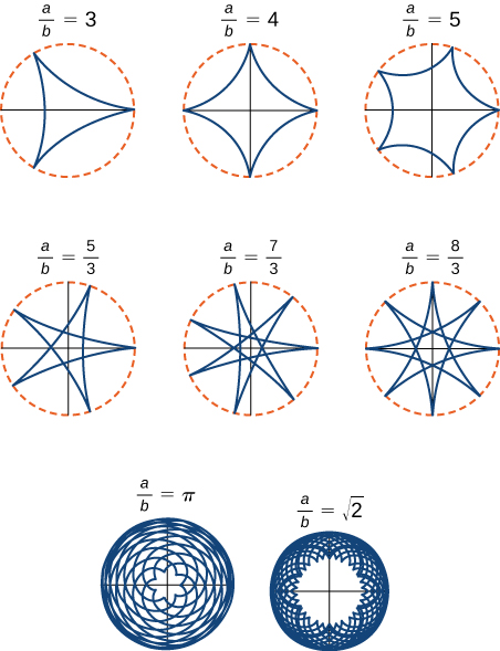
The ratio $\dfrac{a}{b}$ is related to the number of cusps on the graph (cusps are the corners or pointed ends of the graph), as illustrated in Figure $ \PageIndex{10}$. This ratio can lead to some very interesting graphs, depending on whether or not the ratio is rational. Effigy $\PageIndex{9}$ corresponds to $a=4$ and $b=1$. The event is a hypocycloid with four cusps. Effigy $\PageIndex{10}$ shows another possibilities. The last ii hypocycloids accept irrational values for $\dfrac{a}{b}$. In these cases the hypocycloids have an space number of cusps, and then they never return to their starting indicate. These are examples of what are known as infinite-filling curves.

A series of hypocycloids is given. The first is a three pointed star marked a/b = 3. The second is a four pointed star marked a/b = 4. The third is a five pointed star marked a/b = 5. None of these first three figures has lines that cross each other. The fourth figure is a five pointed star but this one has lines which cross each other and looks like the star that children first learn to draw; it is marked a/b = 5/3. A similar sort of star with seven points is next and is marked a/b = 7/3. Then a similar star with eight points is next and is marked a/b = 8/3. The next figure is a complicated series of curves that ultimately creates a small rosette in the middle; this is marked a/b = π. Lastly, there is an even more complicated series of curves that creates a large rosette with sharper florets marked a/b = the square root of 2. — Figure $\PageIndex{10}$: Graph of various hypocycloids corresponding to different values of $a/b$.

The Witch of Agnesi

Many airplane curves in mathematics are named after the people who starting time investigated them, similar the folium of Descartes or the spiral of Archimedes. Withal, maybe the strangest name for a curve is the witch of Agnesi. Why a witch?

Maria Gaetana Agnesi (1718–1799) was i of the few recognized women mathematicians of eighteenth-century Italian republic. She wrote a popular book on analytic geometry, published in 1748, which included an interesting curve that had been studied by Fermat in 1630. The mathematician Guido Grandi showed in 1703 how to construct this curve, which he later called the "versoria," a Latin term for a rope used in sailing. Agnesi used the Italian term for this rope, "versiera," but in Latin, this same word ways a "female goblin." When Agnesi's book was translated into English in 1801, the translator used the term "witch" for the bend, instead of rope. The name "witch of Agnesi" has stuck always since.

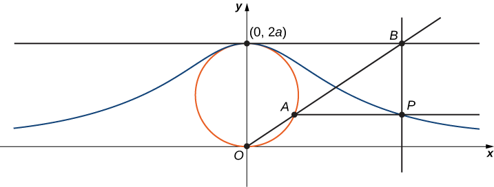
The witch of Agnesi is a curve defined as follows: Commencement with a circle of radius a so that the points $(0,0)$ and $(0,2a)$ are points on the circle (Figure $ \PageIndex{11}$). Let O denote the origin. Choose any other indicate A on the circle, and draw the secant line OA. Let B announce the point at which the line OA intersects the horizontal line through $(0,2a)$. The vertical line through B intersects the horizontal line through A at the bespeak P. As the point A varies, the path that the point P travels is the witch of Agnesi curve for the given circle.

Witch of Agnesi curves have applications in physics, including modeling water waves and distributions of spectral lines. In probability theory, the curve describes the probability density function of the Cauchy distribution. In this project you will parameterize these curves.

A circle with bottom at point O (the origin) and top at point (0, 2a) is drawn. The x axis is drawn from point O, and the y axis is drawn up from point O through (0, 2a). Parallel to the x axis is a line drawn from (0, 2a); it has point B marked to the right. A line from point B to point O passes through the circle at point A. A line is drawn parallel to the x axis from point A, and it forms a right angle with a line drawn down from point B; these lines intersect at point P. There is a curve that is symmetric about the y axis that passes through the point P. This curve has its maximum at (0, 2a) and gently decreases through the point P. — Figure $\PageIndex{eleven}$: As the point $A$ moves around the circumvolve, the point $P$ traces out the witch of Agnesi curve for the given circumvolve.

one. On the figure, characterization the following points, lengths, and angle:

a. $C$ is the indicate on the $x$-axis with the same $x$-coordinate as $A$.

b. $x$ is the $10$-coordinate of $P$, and $y$ is the $y$-coordinate of $P$.

c. $Due east$ is the point $(0,a)$.

d. $F$ is the point on the line segment $OA$ such that the line segment $EF$ is perpendicular to the line segment $OA$.

e. $b$ is the distance from $O$ to $F$.

f. $c$ is the distance from $F$ to $A$.

g. $d$ is the distance from $O$ to $C$.

h. $θ$ is the mensurate of bending $∠COA$.

The goal of this projection is to parameterize the witch using $θ$ as a parameter. To do this, write equations for $10$ and $y$ in terms of only $θ$.

2. Show that $d=\dfrac{2a}{\sin θ}$.

3. Note that $10=d\cos θ$. Prove that $10=2a\cot θ$. When yous do this, you will accept parameterized the $x$-coordinate of the curve with respect to $θ$. If y'all can get a similar equation for $y$, you will accept parameterized the curve.

4. In terms of $θ$, what is the angle $∠EOA$?

5. Show that $b+c=2a\cos\left(\frac{π}{two}−θ\right)$.

6. Testify that $y=2a\cos\left(\frac{π}{2}−θ\correct)\sin θ$.

7. Show that $y=2a\sin^2θ$. Yous accept now parameterized the $y$-coordinate of the curve with respect to $θ$.

8. Conclude that a parameterization of the given witch curve is

\[x=2a\cot θ, \quad y=2a \sin^2θ, \quad\text{for }−∞<θ<∞. \nonumber \]

9. Use your parameterization to evidence that the given witch curve is the graph of the part $f(x)=\dfrac{8a^3}{10^2+4a^2}$.

Travels with My Ant: The Curtate and Prolate Cycloids

Earlier in this section, nosotros looked at the parametric equations for a cycloid, which is the path a point on the edge of a wheel traces every bit the wheel rolls along a straight path. In this project we wait at two different variations of the cycloid, called the curtate and prolate cycloids.

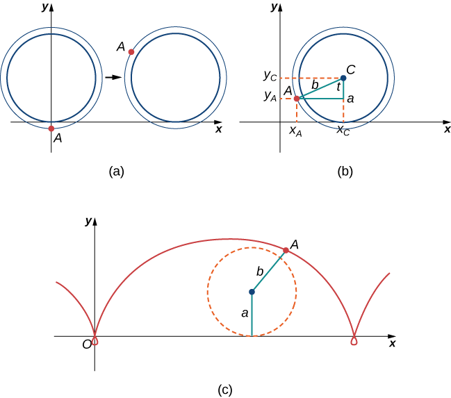
First, let's revisit the derivation of the parametric equations for a cycloid. Recall that we considered a tenacious emmet trying to go habitation by hanging onto the edge of a bicycle tire. We have assumed the ant climbed onto the tire at the very edge, where the tire touches the ground. Equally the cycle rolls, the ant moves with the border of the tire (Figure $\PageIndex{12}$).

Every bit nosotros have discussed, we have a lot of flexibility when parameterizing a bend. In this case we permit our parameter t stand for the bending the tire has rotated through. Looking at Figure $ \PageIndex{12}$, we see that afterward the tire has rotated through an angle of $t$, the position of the center of the wheel, $C=(x_C,y_C)$, is given by

$x_C=at$ and $y_C=a$.

Furthermore, letting $A=(x_A,y_A)$ announce the position of the emmet, nosotros annotation that

$x_C−x_A=a\sin t$ and $y_C−y_A=a \cos t$

Then

\[x_A=x_C−a\sin t=at−a\sin t=a(t−\sin t) \nonumber \]

\[y_A=y_C−a\cos t=a−a\cos t=a(1−\cos t). \nonumber \]

There are two figures marked (a) and (b). Figure a has a circle with point A on the circle at the origin. The circle has — Figure $\PageIndex{12}$: (a) The ant clings to the edge of the bike tire as the tire rolls along the ground. (b) Using geometry to make up one's mind the position of the ant after the tire has rotated through an angle of $t$.

Note that these are the same parametric representations nosotros had earlier, but we take at present assigned a concrete meaning to the parametric variable $t$.

Afterward a while the ant is getting dizzy from going circular and round on the edge of the tire. Then he climbs up one of the spokes toward the center of the wheel. By climbing toward the center of the wheel, the ant has changed his path of motion. The new path has less upwards-and-down motion and is chosen a curtate cycloid (Figure $ \PageIndex{13}$). Every bit shown in the figure, we allow b announce the altitude forth the spoke from the center of the wheel to the ant. As before, nosotros permit t represent the angle the tire has rotated through. Additionally, we let $C=(x_C,y_C)$ represent the position of the center of the wheel and $A=(x_A,y_A)$ correspond the position of the ant.

There are three figures marked (a), (b), and (c). Figure a has a circle with — Effigy $\PageIndex{thirteen}$: (a) The emmet climbs upwardly 1 of the spokes toward the eye of the wheel. (b) The ant's path of motility after he climbs closer to the center of the cycle. This is called a curtate cycloid. (c) The new setup, now that the emmet has moved closer to the center of the bike.

ane. What is the position of the center of the cycle later on the tire has rotated through an angle of $t$?

2. Utilise geometry to discover expressions for $x_C−x_A$ and for $y_C−y_A$.

three. On the footing of your answers to parts 1 and 2, what are the parametric equations representing the curtate cycloid?

One time the ant's caput clears, he realizes that the bicyclist has made a turn, and is at present traveling abroad from his dwelling house. And so he drops off the bike tire and looks around. Fortunately, at that place is a gear up of train tracks nearby, headed back in the right direction. So the emmet heads over to the train tracks to wait. Afterwards a while, a railroad train goes by, heading in the right direction, and he manages to bound up and just catch the edge of the railroad train wheel (without getting squished!).

The ant is still worried about getting silly, but the train wheel is slippery and has no spokes to climb, and then he decides to only hang on to the edge of the wheel and hope for the best. Now, railroad train wheels have a flange to keep the bike running on the tracks. So, in this case, since the ant is hanging on to the very border of the flange, the distance from the center of the bike to the ant is actually greater than the radius of the wheel (Figure $\PageIndex{fourteen}$).

The setup hither is essentially the same as when the ant climbed up the spoke on the bicycle bike. We let b announce the altitude from the center of the wheel to the pismire, and nosotros let t represent the angle the tire has rotated through. Additionally, nosotros let $C=(x_C,y_C)$ correspond the position of the heart of the wheel and $A=(x_A,y_A)$ represent the position of the ant (Effigy $ \PageIndex{14}$).

When the distance from the center of the wheel to the pismire is greater than the radius of the wheel, his path of motion is called a prolate cycloid. A graph of a prolate cycloid is shown in the effigy.

There are three figures marked (a), (b), and (c). Figure a has a circle and a point A that is outside the circle on the y axis (below the origin). The circle is tangent to the x axis at the origin. The circle appears to be travelling to the right on the x axis, with point A being above the x axis in a second image of the circle drawn slightly to the right. Figure b has a circle in the first quadrant with center C. It touches the x axis at xc. A point A is drawn outside the circle and a right triangle is made from this point and point C. The hypotenuse is marked b, the angle at C between A and xc is marked t, and the distance from C to xc is marked a. Lines are drawn to give the x and y values of A as xA and yA, respectively. Similarly, a line is drawn to give the y value of C as yC. Figure c shows the curve that point A would trace out, as the circle travels to the right. It is vaguely sinusoidal with an extra loop at the bottom once per revolution. — Effigy $\PageIndex{xiv}$: (a) The ant is hanging onto the flange of the train wheel. (b) The new setup, at present that the pismire has jumped onto the train wheel. (c) The ant travels along a prolate cycloid.

4. Using the same approach you used in parts 1– 3, observe the parametric equations for the path of motility of the ant.

5. What practice you notice about your answer to function 3 and your answer to part iv?

Find that the ant is actually traveling backward at times (the "loops" in the graph), even though the train continues to move frontwards. He is probably going to be really dizzy past the time he gets home!

Cardinal Concepts

Parametric equations provide a convenient way to describe a curve. A parameter can correspond time or some other meaningful quantity.
It is ofttimes possible to eliminate the parameter in a parameterized curve to obtain a office or relation describing that bend.
There is ever more than than one way to parameterize a curve.
Parametric equations tin can describe complicated curves that are hard or perhaps incommunicable to describe using rectangular coordinates.

Glossary

cycloid: the bend traced by a signal on the rim of a circular wheel as the wheel rolls along a directly line without slippage

cusp: a pointed end or part where two curves meet

orientation: the direction that a indicate moves on a graph as the parameter increases

parameter: an independent variable that both $x$ and $y$ depend on in a parametric bend; usually represented past the variable $t$

parametric curve: the graph of the parametric equations $x(t)$ and $y(t)$ over an interval $a≤t≤b$ combined with the equations

parametric equations: the equations $x=10(t)$ and $y=y(t)$ that ascertain a parametric curve

parameterization of a curve: rewriting the equation of a curve defined by a part $y=f(x)$ every bit parametric equations